How to delete a table in Excel

1. Navigation in the table
2. Selection of parts of the table
3. Adding new rows or columns
4. Deleting rows or columns
5. Move table
6. Sort and filter the table
7. How to create a smart table in Excel
8. Styles and design data in the table
9. Creating tables
10. Deleting tables
11. Delete in Excel

A brief overview of the functionality of tables in Excel was presented. In this article I will give some useful guidelines for working with tables.

Navigation in the table

Selecting cells in a table works the same way as selecting cells within a range. The only difference is the use of the Tab key. Pressing Tab moves the cursor to the cell to the right, but when you reach the last column, pressing Tab moves the cursor to the first cell in the next row.

Selection of parts of the table

As you move your mouse over the table, you may have noticed that it changes its shape. A pointer form helps you select different parts of the table.

• Select the entire column . When you move the mouse pointer to the top of the cell in the title bar, it changes its appearance to an arrow pointing down. Click to select data in a column. Click a second time to select the entire table column (including heading and summary row). You can also press Ctrl + Space (once or twice) to select a column.
• Select the entire line . When you move the mouse pointer to the left side of the cell in the first column, it changes its appearance to an arrow pointing to the right. Click to select the entire row of the table. You can also press Shift + Space to select a row in the table.
• Select the entire table . Move the mouse pointer to the upper left of the upper left cell. When the pointer turns into a diagonal arrow, select a data area in the table. Click a second time to select the entire table (including the title row and summary row). You can also press Ctrl + A (once or twice) to select the entire table.

Right-clicking on a cell in the table displays several selection commands in the context menu.

Adding new rows or columns

To add a new column to the right side of the table, activate the cell in the column to the right of the table and begin data entry. Excel will automatically expand the table horizontally. Similarly, if you enter data in the row below the table, Excel expands the table vertically to include a new row. An exception is the case when the table contains a summary row. When you enter data under this row, the table does not expand. To add rows or columns to a table, right-click and select Insert from the context menu. It allows you to display additional menu items.

When the cell pointer is in the lower right cell of the table, pressing the Tab key inserts a new row at the bottom.

Another way to extend the table is to drag the resize handle that appears in the lower right corner of the table (but only if the entire table is selected). When you move the mouse pointer to the resize marker, the pointer turns into a diagonal line with a double-sided arrow. Click and drag down to add several new rows to the table. Click and drag to the right to add several new columns.

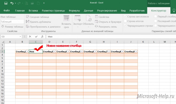
When you insert a new column, the header row contains a general description like a Column1 or Column2 . As a rule, users prefer to change these names to more meaningful ones.

Deleting rows or columns

To delete a row (or column) in a table, select any cell in the row (or column) that will be deleted. If you want to delete multiple rows or columns, select them all. Then right-click and select Delete Table Rows (or Delete Table Columns ).

Move table

To move the table to a new location on the same sheet, move the pointer to any of its borders. When the mouse pointer turns into a cross with four arrows, click and drag the table to a new location. To move a table to another sheet (in the same book or in another book), follow these steps.

1. Press Alt + A twice to select the entire table.
2. Press Ctrl + X to cut selected cells.
3. Activate new sheet and select the top left cell for the table.
4. Press Ctrl + V to paste the table.

Sort and filter the table

The table header row contains a drop-down arrow, which when clicked, shows the sorting and filtering parameters (Fig. 159.1). When a table is filtered, rows that do not meet the filter criteria are temporarily hidden and not counted in the final formulas in the summary row.

The Format as Table tool is a new and useful tool for automatically creating tables in Excel. It speeds up the execution of many tasks and allows you to prevent some errors. It differs radically from the usual cell-formatted cell ranges due to functional tools that work automatically or under user control.

How to create a smart table in Excel

Now the routine work with tables can be performed automatically or semi-automatically. To make sure of this, we start by changing the usual table to automatically formatted table and consider all its properties.

The formulas in the table differ from the usual formulas, but we will consider them in the following lessons.

Styles and design data in the table

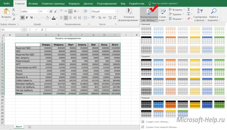
Most quick way Create a table - select the range and press the hot key combination CTRL + T. In this way, the table gets the style assigned by default (in the style gallery it is called “medium 2”). It can be changed to a more suitable style for you. One that you often use in your reports.

Change the formatting style of the table, which is assigned by default:

1. Open the style gallery and right-click on your most frequently used style.
2. From the context menu that appears, select the option: "Default"

Now you can set your own default style. The advantage of this function is especially noticeable when you have to create a lot of tables that must correspond to one or another style.

The size of the table can be easily changed using the marker in its lower right corner.

Expand the table for the new data column. To do this, move the table marker located in the lower right corner to the right, so that another column is added.

By shifting the marker, you can add more columns. All of them will be automatically assigned the headings "Column1", "Column2", etc. The title of the title can easily be changed to the desired values ​​by entering new text into their cells.

The same marker can add new rows to the table, shifting it down. By controlling the marker in any direction, we control the number of rows and columns that the table should contain. You can not only shift the marker diagonally to simultaneously add / delete rows and columns.

Excel sheet is a blank for creating tables (one or several). There are several ways to create tables, and tables created by different ways , provide different possibilities of working with data. About this you can learn from this article.

Creating tables

First, let's talk about creating spreadsheet in a broad sense. What do I need to do:

• on the Excel sheet, enter the names of the columns, rows, data values, insert formulas or functions, if required by the task;
• select the entire filled range;
• turn on all borders .

From the point of view of Excel developers, what you have created is called a range of cells. With this range you can perform various operations: format, sort, filter (if you specify the header row and turn on the Filter on the Data tab) and the like. But you should take care of all the above.

To create a table, as Microsoft programmers understand it, you can choose two ways:

• convert existing range into a table;
• insert a table using Excel.

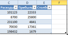
We consider the transformation variant on the example of the table shown in the figure above. Do the following:

• select table cells ;
• use the Insert tab and the Table command;
• in the dialog box, check that the desired range is highlighted, and that the checkbox on the Table with headers option is checked.

The same result, but with the choice of style, one could get if after selecting the range, use the Format as table command on the Home tab.

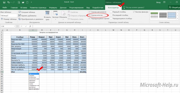
What can you notice right away? The resulting table already has filters (each header has a selection icon from the list). The Designer tab has appeared, the commands of which allow you to manage the table. Other differences are not so obvious. Suppose in the initial version there were no totals under the data columns. Now on the Design tab, you can turn on the totals line , which will lead to the appearance of a new line with buttons for selecting the totals option.

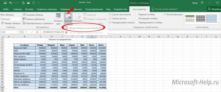
Another advantage of the table is that the filters apply only to its rows, while the data that can be placed in the same column, but outside the table area, is not affected by the filter. This would not have been possible if the filter were applied to what was designated as a range at the beginning of the article. For the table is available the possibility of publishing in SharePoint .

The table can be created immediately, bypassing the filling range. In this case, select the range of empty cells and use any of the above options for creating a table. Headings for such a table are conditional at first, but they can be renamed.

Deleting tables

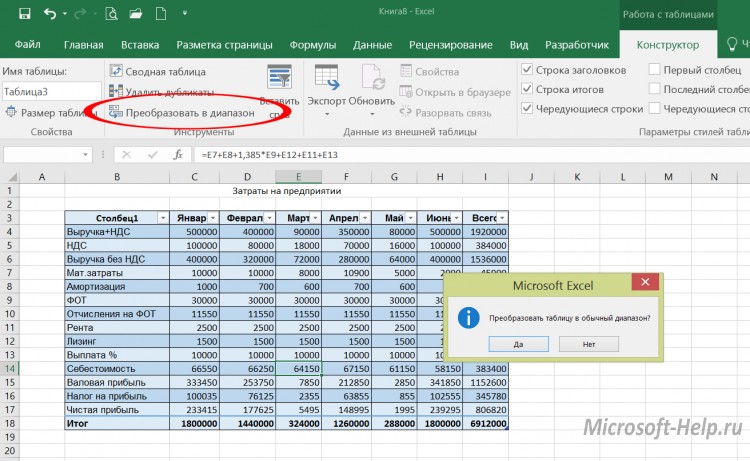
Despite the obvious advantages of tables compared to ranges, it is sometimes necessary to abandon their use. Then on the Design tab, select the Transform to range command (of course, at least one table cell should be selected).

If you need to clear the sheet of data, regardless of whether they were decorated as a range or as a table, then select all the cells with data and use the DELETE key or delete the corresponding columns.

The techniques for creating and deleting tables that you learned from this article will be useful to you in Excel 2007, 2010 and later .

Of all the products Microsoft program Excel is best suited for creating spreadsheets and performing multiple calculations. Many accountants, economists, students use it to build tables and graphs. Even a schoolboy can learn how to work with her. But in the first stages it is impossible to avoid mistakes and then knowledge of how to remove an Excel table, a row or another element will be useful.

Delete in Excel

Unsuccessful work experience can be “erased” like an inscription on a blackboard. The only difference is that it is much easier to do this in the program. Consider everything in order.

• How to remove a row in Excel

It is necessary to select the sheet row to be deleted by clicking on the number pointer on the left side panel. Call the right mouse button floating menu and select the command "delete". The program will remove the string, regardless of whether it contains information or not.

• How to remove blank lines in Excel

In the existing array of information containing empty lines, you should add a column. For convenience, you can place it first. Number the cells in the created column from top to bottom. To do this, in the first register the number “1”, then “hook” the lower right corner of this cell with the mouse while holding down the “ctrl” key and pull down without releasing the “ctrl”. Sort the entries by any column value. All blank lines will be at the bottom of the sheet. Select them and delete. Now sort all the records by the first (specially created) column. Delete the column.

• How to remove Excel spaces

For this operation is responsible for a special function of the program "BATTLE". Applied to cells that have a string format, it removes extra spaces at the beginning or end of the text. Spaces between words function does not delete. In cells of a numeric format, the function removes all spaces.

• How to remove duplicates in Excel

On the sheet, select the desired column, on the panel select the tab “data” - “delete duplicates”. All duplicate column values ​​will be invalidated.

• How to remove duplicate Excel lines

Similar should be done in the presence of the same lines. The “remove duplicates” command will search for absolutely identical string values ​​and delete everything, leaving only one. In this case, select the entire array of values.

• How to delete cells in Excel

Very simple operation. Select the desired cell or array by clicking the left mouse button, with the right we call the floating menu, in which we select the "delete" command. In the dialog box that appears, select the direction of removal: with a shift to the left or up.

• How to remove Excel password

Open password-protected book (file) must be renamed. To do this, select “save as” and in the file saving dialog box, click the “service” menu (lower left corner), then “general settings”. In the fields "Password for opening" and Password for changing "asterisks are deleted. Next, "Ok" and "Save." In the new window, click the "Yes" button to replace the password-protected file with a new one.

• How to delete a sheet in Excel

Sheets in Excel are divided at the bottom of the screen in the form of tabs "Sheet1", "Sheet2" and so on. If you move the mouse cursor over a tab and right-click, a floating menu will appear in which you must select the Delete item. Blank sheet will disappear, and the containing information will ask for confirmation.

• How to remove column in Excel

Select the desired column by clicking on its letter at the top of the window, and right-click. In the floating menu, select "Delete". The column will be deleted, regardless of whether it is empty or contains information.

views